
Introduction
As a budding data scientist, I have been uncertain how I can develop my skills independently. While LLMs today largely allow for many researchers to perform high quality text classification and cleaning, I have struggled with thinking how I can apply these tools.
In an attempt to answer this question, below is the first of a three part series on sentiment analysis. With this series, I’ll explore the limitations of traditional methods, equip myself with the theoretical foundation of LLMs, and eventually integrate an LLM. For this, I have chosen the popular statistical computing language R.
Why choose R? Well, mostly because I wanted re-familiarise myself with the language. Secondly, I wanted to explore how the language fits into the new data analysis paradigm. I’ll further explore this in parts 2 and 3.
The subject of this sentiment analysis is one of my favourite projects, Wikipedia. I find the breadth of its volunteer network and the work they are able to accomplish to be a realisation of what the internet was imagined to be. Therefore, as I set out my journey into sentiment analysis, I thought I would start there.
This post forms the first part of a three-part series on sentiment analysis. This first part will be a naive analysis, where we will simply parse the raw text and use the NRC Emotion Lexicon to get an idea of the sentiment. I will discuss naive sentiment analysis, the data of which I made use, and finally a visualisation of my conclusions. This analysis has been developed in R, to tease out its capabilities in sentiment analysis.
The second part will be an investigation into utilising LLM with R, using the Wikipedia pages of heads of government as a case study. The final part will be a text classification of the Wipageskipedia, finding the highlights and main topics of the text.
What is Sentiment Analysis?
Sentiment analysis is the use of natural language processing and machine learning to systematically identify and classify the emotional quality (positive or negative) of a text. Here is a breakdown of this definition:
- Sentiment: a view or opinion that is held or expressed
- Natural language: language developed organically, for speaking, writing, and reading by humans.
There can be varied workflows for sentiment analysis, depending on what tools you leverage, but here I outline what I think is the essential workflow:
- You collect text data
- Once you’ve processed the data to your ideal atomic unit, attach a sentiment to each unit (the most naive approach is to separate it into individual words).
- You derive analysis scores and benchmarks from the labelled data.
Sentiment Analysis in R
R’s strong statistical analysis capacity is largely supplemented by packages. During the process of implementing my project goals and copy-pasting between drafts, it was easy to lose sight of which packages were useful. Therefore, below I’ve included a list of the packages I’ve used for this sentiment analysis with some explanations on how they were useful to me.
library(readr) # for reading files
library(lubridate) # for working with dates
library(dplyr) # for data frame manipulation
library(stringr) # for working with strings
library(tibble) # having tibble (similar to dataframes) objects
library(tidytext) # this is where stop_words comes from
library(data.table) # helpful for combining data structures to data frames
library(httr2) # for web scraping
This was my first time doing my own sentiment analysis, so my only experience is with R, but I hope in later posts to make comparisons between it and other languages.
Data: Policies, Parsing, and Supplementing
For this sentiment analysis, I wanted to look at the sentiment of the Wikipedia pages of heads of government in the years 2002 and 2020. To achieve, I needed three kind of datasets: heads of government, Wikipedia text, and a word-emotion dictionary.
Two-thirds of the data I needed required some level of web scraping. Previously, I have done small scale web scraping, so I did not so much concern myself with terms of service policies. But, as I was doing this project with this post in mind, I thought let me dot my i’s and cross my t’s here.
Heads of Government
The first step in data mining was looking for heads of government; these are the objects of our analysis. Given the early development of this project, I chose a dataset that presented the most parse-able format. Using Brambor et al.’s The Heads of Government Dataset, I was able to get information on the heads of government in 33 countries in 2002 and 2020. The parsing script for this can be found in naive-parsing-hog.
I was very surprised to see that there was no unified, mostly exhaustive historical dataset of heads of governments. Most of the ones I was able to find were websites, which would require a script for scraping. Perhaps the closest I got to access an exhaustive list with a clean UI was the US’s CIA website, but they don’t allow web scraping as part of their terms of service.
Brambor et al.’s dataset was quite clean, so processing it was quite simple. However, I did spend about 30 minutes confounded by why dplyr::group_by() was not working as I expected it. My understanding of it was that it changed the order of the data. But after hopping through several articles, someone used arrange(). From there, I was able to backtrack my misunderstanding.
-
dplyr::group_by()groups a table into a sections, and data operations (e.g. mean for height of people, grouped by country) are performed on each group separately -
Using
arrange()in conjuction means that we order the rows using our previously defined group.
Wikipedia
Through Wikipedia’s RESTful API, I was able to get the HTML of the desired pages. From there, I just parsed for paragraph elements, <p>, since that was where the majority of relevant content lay.
The workflow for Wikipedia parsing was split into two functions: get_html_from_title for using a head of government’s name to get the HTML from their wikipedia page, and clean_hog_wiki for joining all the paragraphs and filtering out non-alphanumeric characters, paragraph breaks, and Wikipedia’s reference (e.g. [43]).
Following, I converted the text into a dataframe, with the distinct words of the text in one column (one per row) and the name of the head of government in the other.
With the parsing of the data, we were now ready for sentiment analysis.
Supplementing
While I did not do it at this stage, I do feel like it’s worth speaking about supplementing one’s main data source. The main goal behind sentiment analysis is to get an idea of the feelings of the public towards a particular person, event, or organisation. The reason I chose Wikipedia was because I was curious about what a naive sentiment analysis would yield.
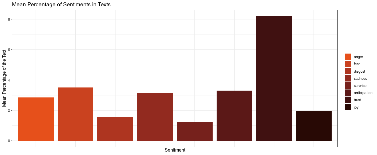
I’ll speak more about it in the conclusions and visualisation section, but I’ll state briefly here that the most common feeling from Wikipedia articles about heads of government was “trust”. At this stage, we can hypothesise about the reasons for this. My main one is that the vocabulary of politics obviously common in pages about a political figure may, removed from context, have the trust sentiment assigned to them, since they speak of structured things.
This immediately shows the pitfalls of a naive analysis of any text: it is more the usage of the words than the words themselves that produce an emotional response. In the second part of this sentiment analysis series, we will explore how we may bridge that gap using R, traditional sentiment analysis and large language models.
Analysis
This section follows the script naive-analysis-hog, explaining the different data objects created and their intended use.
For this naive sentiment analysis, I used the NRC Emotion Lexicon for labelling words with sentiments. For ease, I used the already processed version by Language Technology and Data Analysis Laboratory, which had a shape of 13872x2, loading it with this comamnd:
nrc <- readRDS(url("https://slcladal.github.io/data/nrc.rda", "rb"))
It contains two columns, word and sentiment:
| word | sentiment |
|---|---|
| abacus | trust |
| abandon | fear |
| abandon | negative |
| abandon | sadness |
| abandoned | anger |
| abandoned | fear |
Table 1. nrc.
With hog_annotations, we now have a table that has a head of government, words found in their Wikipedia page (hereafter “text”), and the sentiment of each word. With this, we are now able to derive statistics about the sentiment. I have done it in the following ways:
- The percentage of the prevalence of emotions within a text
- The polarity of a text
The percentage was calculated by getting the frequency of a sentiment across text, including those that were not categorised. From this attribute, we can get a picture of what these pages are written about; we can also see the distribution. The result of this process is percentage_hog, with shape 650x5:
| hog | sentiment | sentiment_freq | words | percentage |
|---|---|---|---|---|
| Abel_Pacheco_de_la_Espriella | anger | 4 | 231 | 1.7 |
| Abel_Pacheco_de_la_Espriella | anticipation | 14 | 231 | 6.1 |
| Abel_Pacheco_de_la_Espriella | fear | 3 | 231 | 1.3 |
| Abel_Pacheco_de_la_Espriella | joy | 7 | 231 | 3 |
| Abel_Pacheco_de_la_Espriella | negative | 8 | 231 | 3.5 |
| Abel_Pacheco_de_la_Espriella | positive | 26 | 231 | 11.3 |
Table 2. percentage_hog.
For the polarity of a text, we used this formula for polarity:
$ \frac{# of positive mentions - # of negative mentions}{total # of mentions} $
This processed resulted in polarity_hog, with shape 66x2 (33 countries, 2 leaders each):
| hog | polarity |
|---|---|
| Abel_Pacheco_de_la_Espriella | 0.191011235955056 |
| Alberto_Fernández | 0.0986159169550173 |
| Alejandro_Toledo | 0.212958551691282 |
| Anders_Fogh_Rasmussen | 0.0787309048178613 |
| Andrés_Manuel_López_Obrador | 0.0672241878417498 |
| Andrés_Pastrana_Arango | 0.15 |
Table 3. polarity_hog.
Results
For each sentiment, we can see that “trust” was the most prevalent emotion in texts, at about 8%.
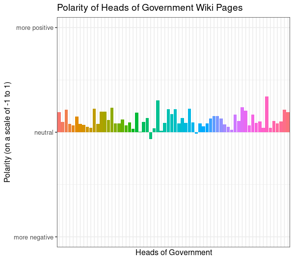
The range of polarity scores can be from $-1$ to $+1$, but there were no values above 0.4 and only two below 0 (Jair Bolsonaro at $-0.0663$ and Kostas Simitis at $-0.0163$), with the majority between $0$ and $0.25$, and a mean of $0.12$. From this naive analysis, one could suppose then that their pages are written in a neutral manner.
Moreover, to show that data analysis is a really a cycle instead of a straight line, I’ll discuss one parsing mistake that only became evident while I was checking the polarity.
Initially, I had a graph that look liked this:
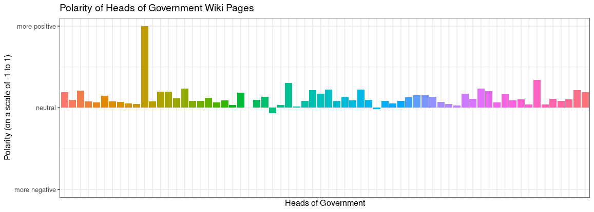
Someone having a polarity of $1$ was extremely odd because it meant that they had only positive words in their Wikipedia page, which was impossible. Going back, I saw that “Carlos Alvarado” (the Costa Rican president in 2020) had only 13 words. By checking the Wikipedia link myself, I saw that the title “Carlos Alvarado” goes to a disambiguation page on Wikipedia. I had to manually modify his name to “Carlos Alvarado Quesada”, which yielded the more accurate:
Conclusion
In this blog post, I discussed a sentiment analysis of the Wikipedia pages of 66 heads of government from 33 countries for years 2002 and 2020. Being the first part of an investigation into sentiment analysis, this served as foray into the space.
It was seen that trust was the most prevalent emotion in the texts, but this can also be explained by the vocabulary of politics being associated with trust. We finally looked at the polarity of each text, and we saw that 95% of the texts were between 0 and 0.25, and the remaining 5% were less than 0.1 outside that boundary.
Despite these simple results, I found this analysis an extremely useful task. I was able to gain familiarity with R using manageable data. I have many more questions about the language now. In this analysis, I mainly used R as a sequential language. On the one hand, as I’ve experienced with other small data science project, defining a function can be more trouble than its worth. But, any project bigger than a semester of work needs a more structured approach. Thus, going forward, I may explore OOP principles within R, and see if it’s appropriate.
Part II is upcoming in March!